Do you know that you can have ggplot in BBC R graphics cookbook? This is an attempt to reproduce https://bbc.github.io/rcookbook/ in python

Todo

Missing Subtitle (plotnine)
Missing Style

Difference between plotnine and ggplot

99% of them are the same, except that in python you have to wrap column names in '', otherwise it will be treated as variable and caused error. Most of the time you just need to wrap a '' or replaced with _ depends on the function.

I tried to produce the same chart with plotnine and altair, and hopefully you will see their difference. plotnine covers 99% of ggplot2, so if you are coming from R, just go ahead with plotnine! altair is another interesting visualization library that base on vega-lite, therefore it can be integrated with website easily. In addition, it can also produce interactive chart with very simple function, which is a big plus!

Setup

# collapse-hide
# !pip install plotnine[all]
# !pip install altair
# !pip install gapminder

from gapminder import gapminder
from plotnine.data import mtcars
from plotnine import *
from plotnine import ggplot, geom_point, aes, stat_smooth, facet_wrap, geom_line
from plotnine import ggplot  # https://plotnine.readthedocs.io/en/stable/
import altair as alt
import pandas as pd
import plotnine
%matplotlib inline

Collecting plotnine[all]
  Using cached https://files.pythonhosted.org/packages/19/da/4d2f68e7436e76a3c26ccd804e1bfc5c58fca7a6cba06c71bab68b25e825/plotnine-0.6.0-py3-none-any.whl
Collecting descartes>=1.1.0 (from plotnine[all])
  Using cached https://files.pythonhosted.org/packages/e5/b6/1ed2eb03989ae574584664985367ba70cd9cf8b32ee8cad0e8aaeac819f3/descartes-1.1.0-py3-none-any.whl
Requirement already satisfied: numpy>=1.16.0 in c:\users\channo.oocldm\appdata\local\continuum\anaconda3\lib\site-packages (from plotnine[all]) (1.16.5)
Requirement already satisfied: matplotlib>=3.1.1 in c:\users\channo.oocldm\appdata\local\continuum\anaconda3\lib\site-packages (from plotnine[all]) (3.1.1)
Requirement already satisfied: statsmodels>=0.9.0 in c:\users\channo.oocldm\appdata\local\continuum\anaconda3\lib\site-packages (from plotnine[all]) (0.10.1)
Requirement already satisfied: pandas>=0.25.0 in c:\users\channo.oocldm\appdata\local\continuum\anaconda3\lib\site-packages (from plotnine[all]) (1.0.3)
Requirement already satisfied: scipy>=1.2.0 in c:\users\channo.oocldm\appdata\local\continuum\anaconda3\lib\site-packages (from plotnine[all]) (1.3.1)
Requirement already satisfied: patsy>=0.4.1 in c:\users\channo.oocldm\appdata\local\continuum\anaconda3\lib\site-packages (from plotnine[all]) (0.5.1)
Collecting mizani>=0.6.0 (from plotnine[all])
  Using cached https://files.pythonhosted.org/packages/e3/76/7a2c9094547ee592f9f43f651ab824aa6599af5e1456250c3f4cc162aece/mizani-0.6.0-py2.py3-none-any.whl
Requirement already satisfied: scikit-learn; extra == "all" in c:\users\channo.oocldm\appdata\local\continuum\anaconda3\lib\site-packages (from plotnine[all]) (0.22.1)
Collecting scikit-misc; extra == "all" (from plotnine[all])
  Using cached https://files.pythonhosted.org/packages/94/4c/e6c3ba02dc66278317778b5c5df7b372c6c5313fce43615a7ce7fc0b34b8/scikit_misc-0.1.1-cp37-cp37m-win_amd64.whl
Requirement already satisfied: cycler>=0.10 in c:\users\channo.oocldm\appdata\local\continuum\anaconda3\lib\site-packages (from matplotlib>=3.1.1->plotnine[all]) (0.10.0)
Requirement already satisfied: kiwisolver>=1.0.1 in c:\users\channo.oocldm\appdata\local\continuum\anaconda3\lib\site-packages (from matplotlib>=3.1.1->plotnine[all]) (1.1.0)
Requirement already satisfied: pyparsing!=2.0.4,!=2.1.2,!=2.1.6,>=2.0.1 in c:\users\channo.oocldm\appdata\local\continuum\anaconda3\lib\site-packages (from matplotlib>=3.1.1->plotnine[all]) (2.4.2)
Requirement already satisfied: python-dateutil>=2.1 in c:\users\channo.oocldm\appdata\local\continuum\anaconda3\lib\site-packages (from matplotlib>=3.1.1->plotnine[all]) (2.8.0)
Requirement already satisfied: pytz>=2017.2 in c:\users\channo.oocldm\appdata\local\continuum\anaconda3\lib\site-packages (from pandas>=0.25.0->plotnine[all]) (2019.3)
Requirement already satisfied: six in c:\users\channo.oocldm\appdata\local\continuum\anaconda3\lib\site-packages (from patsy>=0.4.1->plotnine[all]) (1.12.0)
Requirement already satisfied: palettable in c:\users\channo.oocldm\appdata\local\continuum\anaconda3\lib\site-packages (from mizani>=0.6.0->plotnine[all]) (3.3.0)
Requirement already satisfied: joblib>=0.11 in c:\users\channo.oocldm\appdata\local\continuum\anaconda3\lib\site-packages (from scikit-learn; extra == "all"->plotnine[all]) (0.13.2)
Requirement already satisfied: setuptools in c:\users\channo.oocldm\appdata\local\continuum\anaconda3\lib\site-packages (from kiwisolver>=1.0.1->matplotlib>=3.1.1->plotnine[all]) (41.4.0)
Installing collected packages: descartes, mizani, scikit-misc, plotnine
Successfully installed descartes-1.1.0 mizani-0.6.0 plotnine-0.6.0 scikit-misc-0.1.1
Requirement already satisfied: altair in c:\users\channo.oocldm\appdata\local\continuum\anaconda3\lib\site-packages (4.1.0)
Requirement already satisfied: jinja2 in c:\users\channo.oocldm\appdata\local\continuum\anaconda3\lib\site-packages (from altair) (2.10.3)
Requirement already satisfied: jsonschema in c:\users\channo.oocldm\appdata\local\continuum\anaconda3\lib\site-packages (from altair) (3.0.2)
Requirement already satisfied: entrypoints in c:\users\channo.oocldm\appdata\local\continuum\anaconda3\lib\site-packages (from altair) (0.3)
Requirement already satisfied: numpy in c:\users\channo.oocldm\appdata\local\continuum\anaconda3\lib\site-packages (from altair) (1.16.5)
Requirement already satisfied: toolz in c:\users\channo.oocldm\appdata\local\continuum\anaconda3\lib\site-packages (from altair) (0.10.0)
Requirement already satisfied: pandas>=0.18 in c:\users\channo.oocldm\appdata\local\continuum\anaconda3\lib\site-packages (from altair) (1.0.3)
Requirement already satisfied: MarkupSafe>=0.23 in c:\users\channo.oocldm\appdata\local\continuum\anaconda3\lib\site-packages (from jinja2->altair) (1.1.1)
Requirement already satisfied: pyrsistent>=0.14.0 in c:\users\channo.oocldm\appdata\local\continuum\anaconda3\lib\site-packages (from jsonschema->altair) (0.15.4)
Requirement already satisfied: setuptools in c:\users\channo.oocldm\appdata\local\continuum\anaconda3\lib\site-packages (from jsonschema->altair) (41.4.0)
Requirement already satisfied: six>=1.11.0 in c:\users\channo.oocldm\appdata\local\continuum\anaconda3\lib\site-packages (from jsonschema->altair) (1.12.0)
Requirement already satisfied: attrs>=17.4.0 in c:\users\channo.oocldm\appdata\local\continuum\anaconda3\lib\site-packages (from jsonschema->altair) (19.2.0)
Requirement already satisfied: pytz>=2017.2 in c:\users\channo.oocldm\appdata\local\continuum\anaconda3\lib\site-packages (from pandas>=0.18->altair) (2019.3)
Requirement already satisfied: python-dateutil>=2.6.1 in c:\users\channo.oocldm\appdata\local\continuum\anaconda3\lib\site-packages (from pandas>=0.18->altair) (2.8.0)
Collecting gapminder
  Downloading https://files.pythonhosted.org/packages/85/83/57293b277ac2990ea1d3d0439183da8a3466be58174f822c69b02e584863/gapminder-0.1-py3-none-any.whl
Requirement already satisfied: pandas in c:\users\channo.oocldm\appdata\local\continuum\anaconda3\lib\site-packages (from gapminder) (1.0.3)
Requirement already satisfied: numpy>=1.13.3 in c:\users\channo.oocldm\appdata\local\continuum\anaconda3\lib\site-packages (from pandas->gapminder) (1.16.5)
Requirement already satisfied: pytz>=2017.2 in c:\users\channo.oocldm\appdata\local\continuum\anaconda3\lib\site-packages (from pandas->gapminder) (2019.3)
Requirement already satisfied: python-dateutil>=2.6.1 in c:\users\channo.oocldm\appdata\local\continuum\anaconda3\lib\site-packages (from pandas->gapminder) (2.8.0)
Requirement already satisfied: six>=1.5 in c:\users\channo.oocldm\appdata\local\continuum\anaconda3\lib\site-packages (from python-dateutil>=2.6.1->pandas->gapminder) (1.12.0)
Installing collected packages: gapminder
Successfully installed gapminder-0.1

print(f'altair version: {alt.__version__}')
print(f'plotnine version: {plotnine.__version__}')
print(f'pandas version: {pd.__version__}')

altair version: 4.1.0
plotnine version: 0.6.0
pandas version: 1.0.3

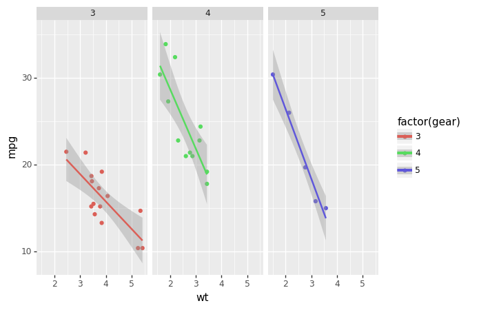
Plotnine Example

(ggplot(mtcars, aes('wt', 'mpg', color='factor(gear)'))
 + geom_point()
 + stat_smooth(method='lm')
 + facet_wrap('~gear'))

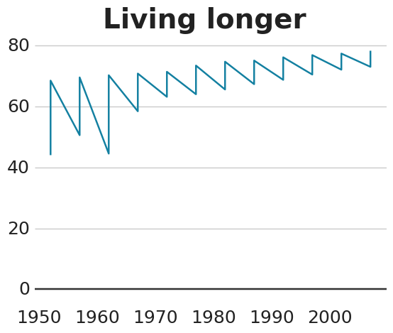
Make a Line Chart

ggplot

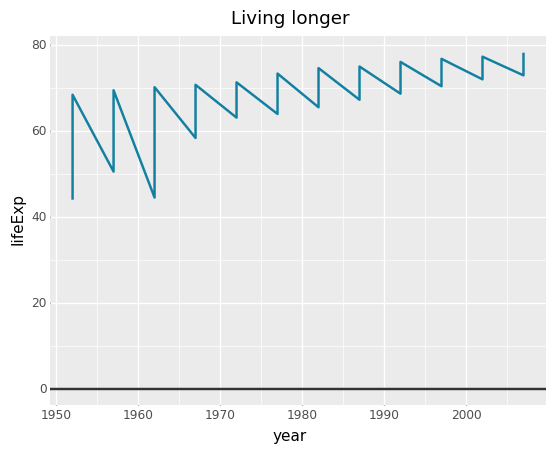
line_df <- gapminder %>%
  filter(country == "Malawi") 

#Make plot
line <- ggplot(line_df, aes(x = year, y = lifeExp)) +
  geom_line(colour = "#1380A1", size = 1) +
  geom_hline(yintercept = 0, size = 1, colour="#333333") +
  bbc_style() +
  labs(title="Living longer",
       subtitle = "Life expectancy in Malawi 1952-2007")

#hide
line_df = gapminder.query(" country == 'Malawi' ")

plotnine

(ggplot(line_df, aes(x='year', y='lifeExp')) +
 geom_line(colour='#1380A1', size=1) +
 geom_hline(yintercept = 0, size = 1, colour='#333333') +
 labs(title='Living longer',
     subtitle = 'Life expectancy in Malawi 1952-2007')
 )

## altair
line = (alt.Chart(line_df).mark_line().encode(
x='year',
y='lifeExp')
.properties(title={'text': 'Living Longer',
                   'subtitle': 'Life expectancy in Malawi 1952-2007'})
)

# hline
overlay = overlay = pd.DataFrame({'y': [0]})
hline = alt.Chart(overlay).mark_rule(color='#333333', strokeWidth=3).encode(y='y:Q')

line + hline

The BBC style

function () 
{
    font <- "Helvetica"
    ggplot2::theme(plot.title = ggplot2::element_text(family = font, 
    size = 28, face = "bold", color = "#222222"), plot.subtitle = ggplot2::element_text(family = font, 
    size = 22, margin = ggplot2::margin(9, 0, 9, 0)), plot.caption = ggplot2::element_blank(), 
    legend.position = "top", legend.text.align = 0, legend.background = ggplot2::element_blank(), 
    legend.title = ggplot2::element_blank(), legend.key = ggplot2::element_blank(), 
    legend.text = ggplot2::element_text(family = font, size = 18, 
        color = "#222222"), axis.title = ggplot2::element_blank(), 
    axis.text = ggplot2::element_text(family = font, size = 18, 
        color = "#222222"), axis.text.x = ggplot2::element_text(margin = ggplot2::margin(5, 
        b = 10)), axis.ticks = ggplot2::element_blank(), 
    axis.line = ggplot2::element_blank(), panel.grid.minor = ggplot2::element_blank(), 
    panel.grid.major.y = ggplot2::element_line(color = "#cbcbcb"), 
    panel.grid.major.x = ggplot2::element_blank(), panel.background = ggplot2::element_blank(), 
    strip.background = ggplot2::element_rect(fill = "white"), 
    strip.text = ggplot2::element_text(size = 22, hjust = 0))
    }
    <environment: namespace:bbplot>

legend_text_align

NameError: name 'legend_text_align' is not defined

def bbc_style():
    font = "Helvetica"
    t = theme(plot_title=element_text(family=font,
                                      size=28, face="bold", color="#222222"),
              #       plot_subtitle=element_text(family=font,
              #                                  size=22, plot_margin=(9, 0, 9, 0)), plot_caption=element_blank(),
              legend_position="top", legend_title_align=0, legend_background=element_blank(),
              legend_title=element_blank(), legend_key=element_blank(),
              legend_text=element_text(family=font, size=18,
                                       color="#222222"), axis_title=element_blank(),

              axis_text=element_text(family=font, size=18,
                                     color="#222222"),
              axis_text_x=element_text(margin={'t': 5, 'b': 10}),
              axis_ticks=element_blank(),
              axis_line=element_blank(), panel_grid_minor=element_blank(),
              panel_grid_major_y=element_line(color="#cbcbcb"),
              panel_grid_major_x=element_blank(), panel_background=element_blank(),
              strip_background=element_rect(fill="white"),
              strip_text=element_text(size=22, hjust=0)
              )
    return t

font = "Helvetica"
theme(plot_title=element_text(family=font,
                                      size=28, face="bold", color="#222222"),
              #       plot_subtitle=element_text(family=font,
              #                                  size=22, plot_margin=(9, 0, 9, 0)), plot_caption=element_blank(),
              legend_position="top", legend_title_align=0, legend_background=element_blank(),
              legend_title=element_blank(), legend_key=element_blank(),
              legend_text=element_text(family=font, size=18,
                                       color="#222222"), axis_title=element_blank(),

              axis_text=element_text(family=font, size=18,
                                     color="#222222"),
              axis_text_x=element_text(margin={'t': 5, 'b': 10}),
              axis_ticks=element_blank(),
              axis_line=element_blank(), panel_grid_minor=element_blank(),
              panel_grid_major_y=element_line(color="#cbcbcb"),
              panel_grid_major_x=element_blank(), panel_background=element_blank(),
              strip_background=element_rect(fill="white"),
              strip_text=element_text(size=22, hjust=0)
              )

<plotnine.themes.theme.theme at 0x163f0ca1508>

The finalise_plot() function does more than just save out your chart, it also left-aligns the title and subtitle as is standard for BBC graphics, adds a footer with the logo on the right side and lets you input source text on the left side.

altair

## altair
line = (alt.Chart(line_df).mark_line().encode(
x='year',
y='lifeExp')
.properties(title={'text': 'Living Longer',
                   'subtitle': 'Life expectancy in China 1952-2007'})
)

# hline
overlay = overlay = pd.DataFrame({'lifeExp': [0]})
hline = alt.Chart(overlay).mark_rule(color='#333333', strokeWidth=3).encode(y='lifeExp:Q')

line + hline

Make a multiple line chart

# hide
# Prepare data
multiline_df = gapminder.query(
    'country == "China" | country =="United States" ')

ggplot

#Prepare data
multiple_line_df <- gapminder %>%
  filter(country == "China" | country == "United States") 

#Make plot
multiple_line <- ggplot(multiple_line_df, aes(x = year, y = lifeExp, colour = country)) +
  geom_line(size = 1) +
  geom_hline(yintercept = 0, size = 1, colour="#333333") +
  scale_colour_manual(values = c("#FAAB18", "#1380A1")) +
  bbc_style() +
  labs(title="Living longer",
       subtitle = "Life expectancy in China and the US")

plotnine

# Make plot
multiline = (
    ggplot(multiline_df, aes(x='year', y='lifeExp', colour='country')) +
    geom_line(colour="#1380A1", size=1) +
    geom_hline(yintercept=0, size=1, color="#333333") +
    scale_colour_manual(values=["#FAAB18", "#1380A1"]) +
      bbc_style() +
    labs(title="Living longer",
         subtitle="Life expectancy in China 1952-2007"))
multiline

findfont: Font family ['Helvetica'] not found. Falling back to DejaVu Sans.
findfont: Font family ['Helvetica'] not found. Falling back to DejaVu Sans.

altair

multiline_altair = (alt.Chart(multiline_df).mark_line().encode(
x='year',
y='lifeExp',
color='country')
.properties(title={'text': 'Living Longer',
                   'subtitle': 'Life expectancy in China 1952-2007'})
)

# hline
overlay = overlay = pd.DataFrame({'lifeExp': [0]})
hline = alt.Chart(overlay).mark_rule(color='#333333', strokeWidth=3).encode(y='lifeExp:Q')

multiline_altair + hline

Make a bar chart

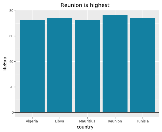
ggplot

#Prepare data
bar_df <- gapminder %>%
  filter(year == 2007 & continent == "Africa") %>%
  arrange(desc(lifeExp)) %>%
  head(5)

#Make plot
bars <- ggplot(bar_df, aes(x = country, y = lifeExp)) +
  geom_bar(stat="identity", 
           position="identity", 
           fill="#1380A1") +
  geom_hline(yintercept = 0, size = 1, colour="#333333") +
  bbc_style() +
  labs(title="Reunion is highest",
       subtitle = "Highest African life expectancy, 2007")

## hide
bar_df = gapminder.query(' year == 2007 & continent == "Africa" ').nlargest(5, 'lifeExp')

plotnine

bars_ggplot = (ggplot(bar_df, aes(x='country', y='lifeExp')) +
  geom_bar(stat="identity",
           position="identity",
           fill="#1380A1") +
  geom_hline(yintercept=0, size=1, colour="#333333") +
#   bbc_style() +
  labs(title="Reunion is highest",
       subtitle="Highest African life expectancy, 2007"))

bars_ggplot

altair

bars_altair = (alt.Chart(bar_df).mark_bar().encode(
x='country',
y='lifeExp',
# color='country'
)
.properties(title={'text': 'Reunion is highest',
                   'subtitle': 'Highest African life expectancy, 2007'})
)

bars_altair

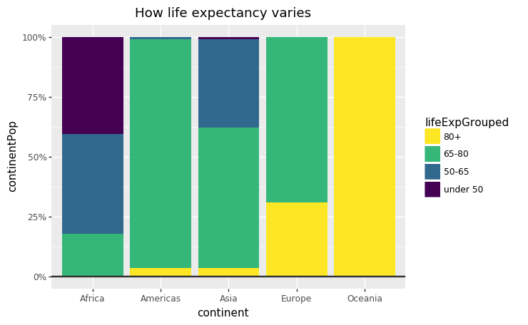
Make a stacked bar chart

Data preprocessing

## collapse-hide
stacked_bar_df = (
    gapminder.query(' year == 2007')
    .assign(
        lifeExpGrouped=lambda x: pd.cut(
            x['lifeExp'],
            bins=[0, 50, 65, 80, 90],
            labels=["under 50", "50-65", "65-80", "80+"]))
    .groupby(
        ['continent', 'lifeExpGrouped'], as_index=True)
    .agg({'pop': 'sum'})
    .rename(columns={'pop': 'continentPop'})
    .reset_index()
)
stacked_bar_df['lifeExpGrouped'] = pd.Categorical(stacked_bar_df['lifeExpGrouped'], ordered=True)

stacked_bar_df.head(6)

	continent	lifeExpGrouped	continentPop
0	Africa	under 50	376100713.0
1	Africa	50-65	386811458.0
2	Africa	65-80	166627521.0
3	Africa	80+	NaN
4	Americas	under 50	NaN
5	Americas	50-65	8502814.0

ggplot

#prepare data
stacked_df <- gapminder %>% 
  filter(year == 2007) %>%
  mutate(lifeExpGrouped = cut(lifeExp, 
                    breaks = c(0, 50, 65, 80, 90),
                    labels = c("Under 50", "50-65", "65-80", "80+"))) %>%
  group_by(continent, lifeExpGrouped) %>%
  summarise(continentPop = sum(as.numeric(pop)))

#set order of stacks by changing factor levels
stacked_df$lifeExpGrouped = factor(stacked_df$lifeExpGrouped, levels = rev(levels(stacked_df$lifeExpGrouped)))

#create plot
stacked_bars <- ggplot(data = stacked_df, 
                       aes(x = continent,
                           y = continentPop,
                           fill = lifeExpGrouped)) +
  geom_bar(stat = "identity", 
           position = "fill") +
  bbc_style() +
  scale_y_continuous(labels = scales::percent) +
  scale_fill_viridis_d(direction = -1) +
  geom_hline(yintercept = 0, size = 1, colour = "#333333") +
  labs(title = "How life expectancy varies",
       subtitle = "% of population by life expectancy band, 2007") +
  theme(legend.position = "top", 
        legend.justification = "left") +
  guides(fill = guide_legend(reverse = TRUE))

plotnine

# create plot
stacked_bar_ggplot = (
    ggplot(stacked_bar_df,
           aes(x='continent',
               y='continentPop',
               fill='lifeExpGrouped')
           ) +
    geom_bar(stat="identity",
             position="fill") +
    #   bbc_style() +
    scale_y_continuous(labels=lambda l: ["%d%%" % (v * 100) for v in l]) +
    scale_fill_cmap_d(direction=-1) +  # scale_fill_viridis_d
    geom_hline(yintercept=0, size=1, colour="#333333") +
    labs(title="How life expectancy varies",
         subtitle="% of population by life expectancy band, 2007") +

    guides(fill=guide_legend(reverse=True)))

stacked_bar_ggplot

C:\Users\CHANNO.OOCLDM\AppData\Local\Continuum\anaconda3\lib\site-packages\plotnine\scales\scale.py:91: PlotnineWarning: scale_fill_cmap_d could not recognise parameter `direction`
  warn(msg.format(self.__class__.__name__, k), PlotnineWarning)
C:\Users\CHANNO.OOCLDM\AppData\Local\Continuum\anaconda3\lib\site-packages\plotnine\layer.py:433: PlotnineWarning: position_stack : Removed 7 rows containing missing values.
  data = self.position.setup_data(self.data, params)

# create plot
stacked_bar_ggplot = (
    ggplot(stacked_bar_df,
           aes(x='continent',
               y='continentPop',
               fill='lifeExpGrouped')
           ) +
    geom_bar(stat="identity",
             position="fill") +
    #   bbc_style() +
    scale_y_continuous(labels=lambda l: ["%d%%" % (v * 100) for v in l]) +
    scale_fill_cmap_d(direction=-1) +  # scale_fill_viridis_d
    geom_hline(yintercept=0, size=1, colour="#333333") +
    labs(title="How life expectancy varies",
         subtitle="% of population by life expectancy band, 2007") +

    guides(fill=guide_legend(reverse=True)))

stacked_bar_ggplot

C:\Users\CHANNO.OOCLDM\AppData\Local\Continuum\anaconda3\lib\site-packages\plotnine\scales\scale.py:91: PlotnineWarning: scale_fill_cmap_d could not recognise parameter `direction`
  warn(msg.format(self.__class__.__name__, k), PlotnineWarning)
C:\Users\CHANNO.OOCLDM\AppData\Local\Continuum\anaconda3\lib\site-packages\plotnine\layer.py:433: PlotnineWarning: position_stack : Removed 7 rows containing missing values.
  data = self.position.setup_data(self.data, params)

altair

stacked_bar_altair = (
    alt.Chart(stacked_bar_df)
    .mark_bar()
    .encode(x='continent',
            y=alt.Y('continentPop', stack='normalize',
                    axis=alt.Axis(format='%')),
            fill=alt.Fill('lifeExpGrouped', scale=alt.Scale(scheme='viridis')))
    .properties(title={'text': 'How life expectancy varies',
                       'subtitle': '% of population by life expectancy band, 2007'}
                )
)

overlay = overlay = pd.DataFrame({'continentPop': [0]})
hline = alt.Chart(overlay).mark_rule(
    color='#333333', strokeWidth=2).encode(y='continentPop:Q')


stacked_bar_altair + hline

Make a grouped bar chart

# hide
grouped_bar_df = (
    gapminder[[
        'country', 'year', 'lifeExp'
    ]].query(' year == 1967 | year == 2007 ')
    .pivot_table(
        index=['country'], columns='year',
        values='lifeExp')
    .assign(gap=lambda x: x[2007] - x[1967])
    .nlargest(5, 'gap')
    .reset_index()
    .melt(value_vars=[1967, 2007],
          id_vars=['country', 'gap'],
      value_name='lifeExp')
)

grouped_bar_df

	country	gap	year	lifeExp
0	Oman	28.652	1967	46.988
1	Vietnam	26.411	1967	47.838
2	Yemen, Rep.	25.714	1967	36.984
3	Indonesia	24.686	1967	45.964
4	Libya	23.725	1967	50.227
5	Oman	28.652	2007	75.640
6	Vietnam	26.411	2007	74.249
7	Yemen, Rep.	25.714	2007	62.698
8	Indonesia	24.686	2007	70.650
9	Libya	23.725	2007	73.952

ggplot

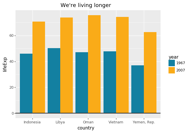
#Prepare data
grouped_bar_df <- gapminder %>%
  filter(year == 1967 | year == 2007) %>%
  select(country, year, lifeExp) %>%
  spread(year, lifeExp) %>%
  mutate(gap = `2007` - `1967`) %>%
  arrange(desc(gap)) %>%
  head(5) %>%
  gather(key = year, 
         value = lifeExp,
         -country,
         -gap) 
  
#Make plot
grouped_bars <- ggplot(grouped_bar_df, 
                       aes(x = country, 
                           y = lifeExp, 
                           fill = as.factor(year))) +
  geom_bar(stat="identity", position="dodge") +
  geom_hline(yintercept = 0, size = 1, colour="#333333") +
  bbc_style() +
  scale_fill_manual(values = c("#1380A1", "#FAAB18")) +
  labs(title="We're living longer",
       subtitle = "Biggest life expectancy rise, 1967-2007")

plotnine

# Make plot
grouped_bars_ggplot = (ggplot(grouped_bar_df,
                       aes(x='country',
                           y='lifeExp',
                           fill='year')) +
                geom_bar(stat="identity", position="dodge") +
                geom_hline(yintercept=0, size=1, colour="#333333") +
#                 bbc_style() +
                scale_fill_manual(values=("#1380A1", "#FAAB18")) +
                labs(title="We're living longer",
                     subtitle="Biggest life expectancy rise, 1967-2007"))

grouped_bars_ggplot

altair

grouped_bars_altair = (
    alt.Chart(grouped_bar_df)
    .mark_bar()
    .encode(x='year:N',
            y='lifeExp',
color=alt.Color('year:N', scale=alt.Scale(range=["#1380A1", "#FAAB18"])),
           column='country:N')
    .properties(title={'text': "We're living longe",
                       'subtitle': 'Biggest life expectancy rise, 1967-2007'}
                )
)

grouped_bars_altair

Make changes to the legend

## hide

plotnine

# Remove the Legend
multiline + guides(colour=False)

multiline + theme(legend_position = "none")

from plotnine import unit

ImportError: cannot import name 'unit' from 'plotnine' (C:\Users\CHANNO.OOCLDM\AppData\Local\Continuum\anaconda3\lib\site-packages\plotnine\__init__.py)

# Change position of the legend
x=multiline + theme(
  axis_ticks_major_x = element_line(color = "#333333"),
  axis_ticks_length =  0.26)

x

altair

Make changes to the axes

## hide

ggplot

plotnine

altair

Add annotations

## hide

ggplot

plotnine

altair

Work with small multiples

## hide

ggplot

plotnine

altair

Do something else entirely

## hide

ggplot

plotnine

altair

Make a dumbbell chart

# hide
dumbbell_chart_df = (
    gapminder[[
        'country', 'year', 'lifeExp'
    ]].query(' year == 1967 | year == 2007 ')
    .pivot_table(
        index=['country'], columns='year',
        values='lifeExp')
    .assign(gap=lambda x: x[2007] - x[1967])
    .nlargest(10, 'gap')
)

dumbbell_chart_df

year	1967	2007	gap
country
Oman	46.988	75.640	28.652
Vietnam	47.838	74.249	26.411
Yemen, Rep.	36.984	62.698	25.714
Indonesia	45.964	70.650	24.686
Libya	50.227	73.952	23.725
Gambia	35.857	59.448	23.591
Saudi Arabia	49.901	72.777	22.876
Nepal	41.472	63.785	22.313
Egypt	49.293	71.338	22.045
Tunisia	52.053	73.923	21.870

ggplot

#Prepare data
dumbbell_df <- gapminder %>%
  filter(year == 1967 | year == 2007) %>%
  select(country, year, lifeExp) %>%
  spread(year, lifeExp) %>%
  mutate(gap = `2007` - `1967`) %>%
  arrange(desc(gap)) %>%
  head(10)

ggplot(hist_df, aes(lifeExp)) +
  geom_histogram(binwidth = 5, colour = "white", fill = "#1380A1") +
  geom_hline(yintercept = 0, size = 1, colour="#333333") +
  bbc_style() +
  scale_x_continuous(limits = c(35, 95),
                     breaks = seq(40, 90, by = 10),
                     labels = c("40", "50", "60", "70", "80", "90 years")) +
  labs(title = "How life expectancy varies",
       subtitle = "Distribution of life expectancy in 2007")

plotnine

Not available with plotnine.

altair

dumbbell_chart_altair = (
alt.Chart(dumbbell_chart_df).
    mark_rule()
)

dumbbell_chart_altair

()